A Heuristic Measure for Estimating the Complexity of Novel Coronavirus
Posted on 06 Aug 2020; 03:00 AM IST. Last Updated 09 Aug 2020; 07:30 PM IST.Summary: The novel coronavirus (covid-19), threw many challenges to all across the board, from health care professionals to data analysts. From the perspective of data analysis, the challenge is to interpret the current situation or complexity of the disease, from daily or cumulative figures. When only the number of infections discovered was used as a measure, the Unites States of America (USA), stood at the top of the list. The outcome undermined the gut feeling of many administrators, and the President of USA expressed such a feeling, several times. This article provides an intuition into a heuristic measure, and attempts to estimate the complexity of the disease, in terms of the heuristic measure.
The Novel Coronavirus (covid-19) is currently estimated by a measure called positivity rate. This measure is expressed as:
positivity rate (r) =
number of positive cases (p) /
number of tests performed (t); - - - (1)
Positivity rate is a decent measure, but it alone is insufficient to estimate the complexity of the disease. Intuitively, when a more populous country, has the same positivity rate as a less populous country, then the more populous country is at a disadvantage.
The heuristic measure
It is possible to tie in both population and positivity rate into a single measure, as described below.
heuristic measure (u) =
positivity rate (r) /
number tests per unit population (m); - - - (2)
where,
number tests per unit population (m) =
number of tests performed (t) /
population count (n);
From the above two equations, we can deduce, the heuristic measure as:
u = (p / t) / (t / n)
= (p * n) / (t * t)
= pn / t2; - - - (3)
The heuristic measure identifies the complexity of the system. Technically, we multiply the positivity rate with a factor (n / t), and describe the result as complexity. The complexity measure increases modestly, if the tests were proportional to the population. If there is a serious shortcoming in the number of tests with respect to population, then the complexity sky rockets, just as we would expect it to behave.
Examples of heuristic measure
The following examples demonstrate, how the heuristic measure can be applied to establish the complexity of the disease.
Consider a country with a population of 1 million, which has tested 10% of its population or 100,000. Let us assume that 10% of those tested i.e 10,000, were found to be positive for the disease.
In the above example, we have
n = 1,000,000; t = 100,000; p = 10,000; and
u = (10,000 * 1,000,000) / (100,000 * 100,000)
= 1.0;
A few more example scenarios, and their complexities are presented below.
i) n = 500,000; t = 100,000; p = 10,000; and
u = (10,000 * 500,000) / (100,000 * 100,000)
= 1 / 2 = 0.5;
ii) n= 100,000; t = 100,000; p = 10,000; and
u = (10,000 * 100,000) / (100,000 * 100,000)
= 1 / 10 = 0.1;
iii) n= 2,000,000; t = 100,000; p = 10,000; and
u = (10,000 * 2,000,000) /
(100,000 * 100,000)
= 2 / 1 = 2.0;
iv) n = 1,000,000; t = 100,000; p = 20,000; then
u = (20,000 * 1,000,000) /
(100,000 * 100,000)
= 2 / 1 = 2.0;
The complexity increases, when the population increases, even when the positivity rate remains constant. Similarly, the complexity increases, when the positivity rate increases, even when the population remains constant.
It may be noted that when the number of tests approach the population size (t -> n), then the heuristic measure or complexity measure "u" approaches the positivity rate (p / t). Since (t -> n), the complexity "u" -> (p / t) -> (p / n), or the positive fraction of the population.
An anomaly in the complexity measure
An anomaly in the complexity measure, is described below.
Assume that we tested every person in a country, and every person tested positive. In such a case, we have p = n = t, and u = 1.0.
In view of the anomaly in the complexity measure, the following norms was invented.
The Norms for Complexity Measure
The following norms could serve as guidance on how Complexity measure can be employed in a real life scenario.
First Norm: The ratio q = ( p / n ), which is count of positive over population size, and represents the percentage of positive population, is regarded as the quality factor. This factor must remain low (between 1 and 10%), throughout the analysis, or period of study.
Second Norm: A complexity measure of u = 1.0 or less, when q is in between 1 and 10%, is considered a reasonable achievement or containment of the disease. A complexity measure of u > 1.0 is regarded as under achievement, and u < 1.0 is regarded as over achievement.
It may be noted that the complexity measure can not be used as a norm independently by itself, but can be used as a reliable indicator, when the first norm holds.
A real life scenario
The above theory was applied to a real life novel coronavirus scenario, and the complexity measures are evaluated and compared. The raw data for the analysis was obtained from Worldometer on 05 Aug 2020.
Case - 1: Complexity measure of Novel Coronavirus in USA
From the data sheet, we note
n = 331,187,544; t = 61,692,067; p = 4,924,734;
u = ( 4,924,734 * 331,187,544) /
( 61,692,067 * 61,692,067 )
= 0.43;
Case - 2: Complexity measure of Novel Coronavirus in Brazil
From the data sheet, we note
n = 212,702,448; t = 13,329,028; p = 2,808,076;
u = ( 2,808,076 * 212,702,448) /
( 13,329,028 * 13,329,028 )
= 3.36;
Case - 3: Complexity measure of Novel Coronavirus in India
From the data sheet, we note
n = 1,381,270,916; t = 21,484,402; p = 1,958,592;
u = ( 1,958,592 * 1,381,270,916) /
( 21,484,402 * 21,484,402 )
= 5.86;
Case - 4: Complexity measure of Novel Coronavirus in Russia
From the data sheet, we note
n = 145,940,583; t = 29,400,000; p = 866,627;
u = ( 866,627 * 145,940,583) /
( 29,400,000 * 29,400,000 )
= 0.15;
Case - 5: Complexity measure of Novel Coronavirus in Japan
From the data sheet, we note
n = 126,437,965; t = 877,134; p = 39,858;
u = ( 39,858 * 126,437,965) /
( 877,134 * 877,134 )
= 6.55;
What we discovered so far is that although USA, Brazil and India are listed as the top three countries in the number of coronavirus infections, the complexity of the situation is very different for the three countries.
It may be noted that complexity of USA is far below Brazil and Brazil in turn has less complexity than India.
As expected, Russia fares even better than USA in terms of complexity, since Russia is more spacious than USA, and the population density is low (automatic social distancing).
Finally, Japan (which has a severe space constraint), has a higher complexity than India.
Further Analysis
If we use positivity rate as a measure, then we have the following scenario.
r ( Usa ) = 4,924,734 / 61,692,067 = 0.08
r ( India ) = 1,958,592 / 21,484,402 = 0.09
r ( Japan ) = 39,858 / 877,134 = 0.05
As per the positivity rate, Japan is in a better position than USA or India, and USA and India are approximately in the same kind of scenario.
Complexity measure presents a different picture, and rates USA as less complex than India or Japan, and Japan as more complex than India.
The following presents a generalized scheme for analyzing the complexity of a scenario.
1) First we note that u = pn / t2; which could be rewritten as:
pn = ut2; - - - (4)
2) Next we note that number of tests is a percentage of population. For example,
t = n / 2 => half the population is tested;
t = n / 3 => a third of the population is tested; and so on . . .
In general, we could write t = n / k;
where, "k" is some portion of the population.
3) Substituting t = n / k, in equation (4), we get
pn = u n2 / k2
=> p = (u / k2) * n - - - (5)
=> ( p / n ) = (u / k2)
=> k2 = ( u / ( p / n ) )
=> k = sqrt ( ( u * 100 ) / q ) - - - (6)
A few important questions that could arise are listed below.
a) when do we stop testing, and
b) what is excess testing?
The most honest answer for the first question is "data analysis" cannot tell when testing should be stopped.
With regard to the second question of excess testing, data analysis could provide a few pointers, which are discussed in the next section.
Under Testing and Excess Testing
As suggested in the norms for complexity measure, when the value of "u" is above 1.0, it implies under testing, and we need to perform more tests, which increase "t", and possibly "p" (or q).
Similarly, we can recognize excess testing, when the complexity measure "u" goes below 1.0;
Excess testing in reality is good for disease monitoring. It increases confidence that the disease is under control.
Data analysis could tell when excess testing scenario kicks in, and how much could be regarded as excess testing.
Before going further, it may be noted that norms for determining "excess testing" are not hard norms, but are soft norms.
We consider the complexity measure u = 1.0 as a reference point. This is a soft norm invented by the author of the article.
For the complexity measure of u = 1.0, we can easily calculate k-values, for various q-values, using equation (6).
For example, for u = 1.0 and q = 1.0, we have
k = sqrt ( ( 1.0 * 100 ) / 1.0 )
= 10
k = 10 => testing 10% of the population.
for u = 1.0 and q = 10.0, we have
k = sqrt ( ( 1.0 * 100 ) / 10.0 )
= 3.16
k = 3.16 => testing 31.65% or one third of the population.
When the complexity measure "u" goes below 1.0, we compare the number of tests for current u-value, with the number of tests for u = 1.0. This would reveal the excess tests, in the current scenario.
The following example, illustrates the technique.
From the above section, we note USA has:
n = 331,187,544; t = 61,692,067; p = 4,924,734; u = 0.43; q = p / n = 1.5%;
Since u is < 1.0, we consider this scenario as excess testing.
We can compute reference "k", for u = 1.0, and q = 1.5%, for USA, as follows :
reference-k = sqrt ( (1.0 * 100) / 1.5 ) = 8.2
The number of reference tests for u = 1.0, for USA, would be:
reference-t = n / reference-k
= 41,398,443
= 41 million
Actual tests performed are:
actual-t = 61,692,067
= 61 million
The logical intuition behind the variance between the reference tests and actual tests may be explained as follows.
First we note that, we kept q (= 1.5% as constant ), for computing the reference tests. Conversely, the reference prescribed that 41 million tests would suffice to hold q at 1.5%, but in the actual real life, we had to conduct 61 million tests to arrive at a positive count, which would yield q = 1.5%.
The above variance could be due to two issues -
a) It is increasingly difficult to spot the disease, because the disease is under control.
b) The testing is poorly coordinated.
We could ignore the second case, since u is already below 1.0, which means the disease is under control, and accept the first case, that it is increasingly difficult to spot the disease.
In the above example, for USA, the excess testing percentage is given as:
( actual-t - reference-t ) / actual-t
= ( 61 million - 41 million ) / 61 million
= 32.79%
Conclusion
In conclusion, it may be stated that the positive percentage of the population q = p / n, is the final indicator for the performance of a country, in its fight against coronavirus. While "q" by itself is not a great indicator, it turns out to be a great indicator, when the complexity measure "u" is reduced to 1.0. It may be noted that the definition of "u", implies that "q" must lie within the limits of 1 to 10%.
From the computations shown above, it can be seen that only USA and Russia have a complexity measure < 1.0.
The final q-value for USA is 1.5%, where as it is only 0.6% for Russia.
The prevalence of the disease appears to be based on the racial profile of the population. The following were observed based on crude estimates:
a) European : 0.2% to 0.5% (Germany, France, Denmark, Serbia, UK)
b) Asian & Mediterranean : 0.8% to 1.0% (Saudi, Israel, Singapore)
c) Hispanic : 1.4% to 2.0%
d) African : no reliable data
From the raw data given in previous section, we can easily observe that Japan has a q-value of 0.03%, and India has a q-value of 0.14%, and the complexities are 6.55, and 5.86 respectively. The q-value, for Japan and India, when the complexity is reduced to 1.0, can be computed as: 0.2% and 0.8% respectively. The final q-value of 0.8% for India is stunning, and correlates very well with the Asian neighbours.
Finally, there are a few countries with very low prevalence (q-value < 0.1%), and some of these are listed below.
Martinique, Mauritius, Mongolia, Morocco, New Caledonia, New Zealand, Cuba
Except Mongolia, and Morocco the rest are islands. Morocco is not an island, but it is a sea facing nation. It could be a topic of interest for health care professionals to investigate, why Cuba has very low prevalence, whereas Brazil has high prevalence.
The conclusion is, if the island nations are excluded, then there are no major differences in the manner, the rest of the nations are fighting covid-19.
Remarks
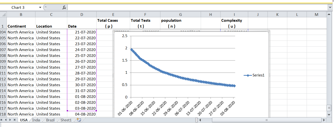
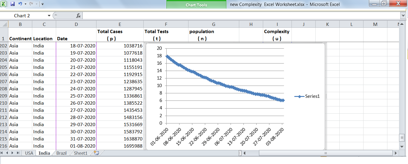
A plot of complexity of USA (weblink) from June 2020 to August 2020, using data from European CDC, revealed a steady exponential decline in complexity. A similar complexity plot for India (weblink), revealed a steady linear decline in complexity and how hard India is fighting with the novel coronavirus.
An algorithm to compute the final q-value, for u = 1.0, is available at this weblink.